Flower Classification with TPUs
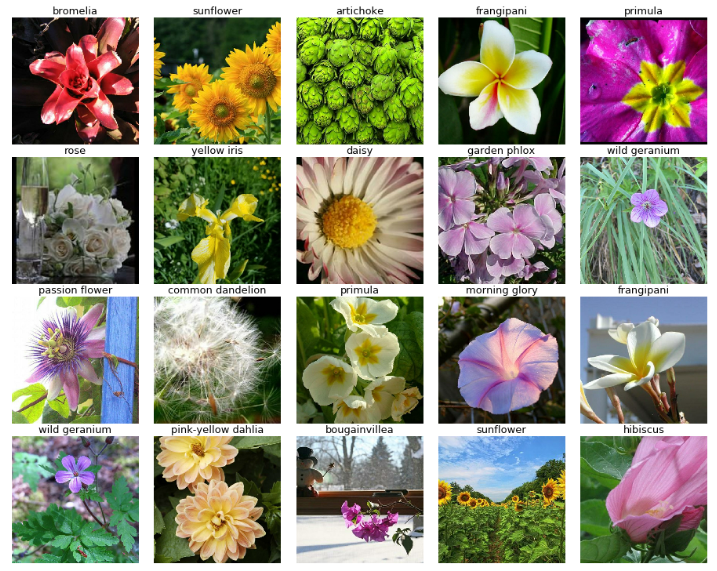
There are over 5,000 species of mammals, 10,000 species of birds, 30,000 species of fish – and astonishingly, over 400,000 different types of flowers. In this competition, we are challenged to build a machine learning model that identifies the type of flowers in a dataset of images over 104 types.
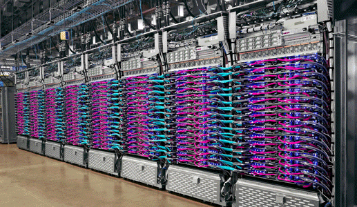
Tensor Processing Units (TPUs)
TPUs are powerful hardware accelerators specialized in deep learning tasks. Cloud TPU is the custom-designed machine learning ASIC that powers Google products like Translate, Photos, Search, Assistant, and Gmail. They were developed and first used by Google to process large image databases. This competition is designed to give TPUs a try.
Data Description
Images are provided in TFRecord format, a container format frequently used in Tensorflow to group data files for optimal training performace. Each file contains the id, label and image.
- 12753 training images
- 3712 validation images
- 7382 unlabeled test images
Recipe for accuracy 95+ [code on Kaggle]
Do not waste your time on simple data loading and inspecting code. Use the getting started notebook.
1- Use Transfer Learning with fine tuning.
To avoid over-fitting, use small networks such as DenseNet used here.
First, freeze the weights of the pretrained network and trian only the added layers.
with strategy.scope():

    pretrained_model = tf.keras.applications.DenseNet201(weights='imagenet', include_top=False ,input_shape=[*IMAGE_SIZE, 3])
    pretrained_model.trainable = False # freeze

    model = tf.keras.Sequential([
        pretrained_model,
        tf.keras.layers.GlobalAveragePooling2D(),
        tf.keras.layers.Dense(len(CLASSES), activation='softmax')
    ])
Second, fine tune the whole network.
pretrained_model.trainable = True
model.compile(
    optimizer='adam',
    loss = categorical_smooth_loss,
    metrics=['categorical_accuracy']
)
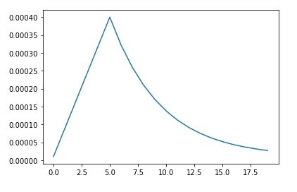
2- Use learning rate scheduling, for more stable training.
High initial learning rates can make loss explode. It is usually better linearly to increase learning rate from very small value over the first ~5000 iterations. Moreover, if we increase the batch size by N, also scale the initial learning rate by N. Goyal et al, Accurate, Large Minibatch SGD: Training ImageNet in 1 Hour.
LR_START = 0.00001
LR_MAX = 0.00005 * strategy.num_replicas_in_sync
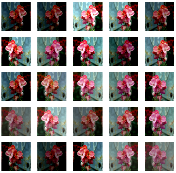
3- Use reasonable data augmentation
def data_augment(image, label):
    # data augmentation. Thanks to the dataset.prefetch(AUTO) statement in the next function (below),
    # this happens essentially for free on TPU. Data pipeline code is executed on the "CPU" part
    # of the TPU while the TPU itself is computing gradients.
    image = tf.image.random_flip_left_right(image)
    image = tf.image.random_hue(image, 0.05)
    image = tf.image.random_contrast(image, 0.5, 1.5)
    image = tf.image.random_brightness(image, 0.25)
    # also try random_saturation, resize and random_crop
    return image, label
4- Use Label smoothing to have a better generalization.
Label smoothing is a mechanism for encouraging the model to be less confident. Instead of minimizing cross-entropy with hard targets (one-hot encoding), we minimize it using soft targets.
def categorical_smooth_loss(y_true, y_pred, label_smoothing=0.1):
    loss = tf.keras.losses.categorical_crossentropy(y_true, y_pred, label_smoothing=label_smoothing)
    return loss
model.compile(
    optimizer='adam',
    loss = categorical_smooth_loss,
    metrics=['categorical_accuracy']
)
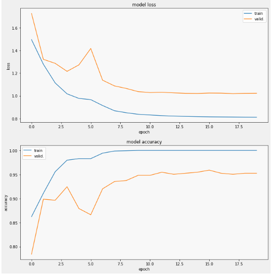
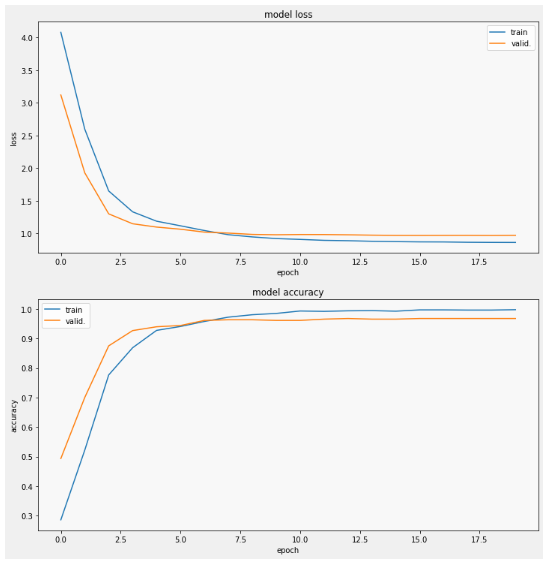
Results
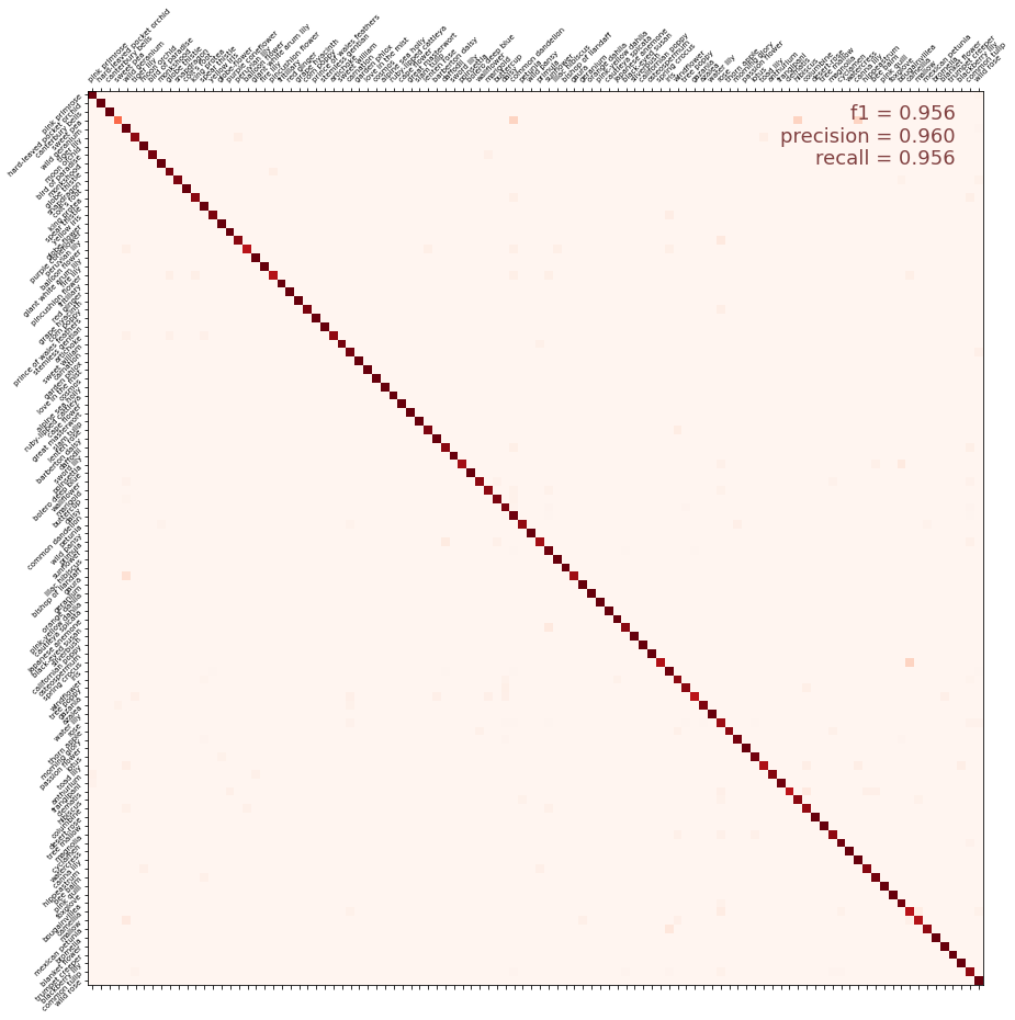
More for accuracy 96+ [code on Kaggle]
Use simple Ensemble of DenseNet201 and EfficientNetB7
Instead of one network, we train two and then combine their probability distributions.
- Find best weight between models (can be another model!)
scores = []
for alpha in np.linspace(0,1,100):
    cm_probabilities = alpha*cm_probabilities1+(1-alpha)*cm_probabilities2
    cm_predictions = np.argmax(cm_probabilities, axis=-1)
    scores.append(accuracy_score(cm_correct_labels, cm_predictions))
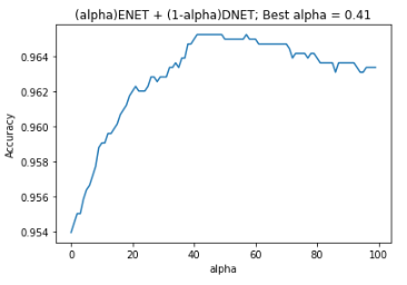
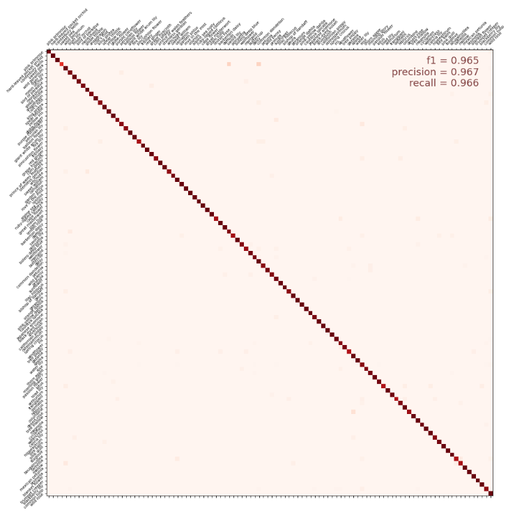
Results
Next Steps:
- Use more Networks (EfficientNet)
- More data augmentation (Rotation with small angles)
- Try Focal Loss with different settings
- Try label smoothing with different settings
- Train Ensemble as one network, end to end