Chest X-ray (Covid-19 & Pneumonia)

COVID-19 (coronavirus disease 2019) is an infectious disease caused by severe acute respiratory syndrome coronavirus 2 (SARS-CoV-2), a strain of coronavirus. The first cases were seen in Wuhan, China, in late December 2019 before spreading globally. The current outbreak was officially recognized as a pandemic by the World Health Organization (WHO) on 11 March 2020. Currently Reverse transcription polymerase chain reaction (RT-PCR) is used for diagnosis of the COVID-19. X-ray machines are widely available and provide images for diagnosis quickly so chest X-ray images can be very useful in early diagnosis of COVID-19. In this classification project, there are three classes:

COVID19
PNEUMONIA
NORMAL

cover

1) Data description

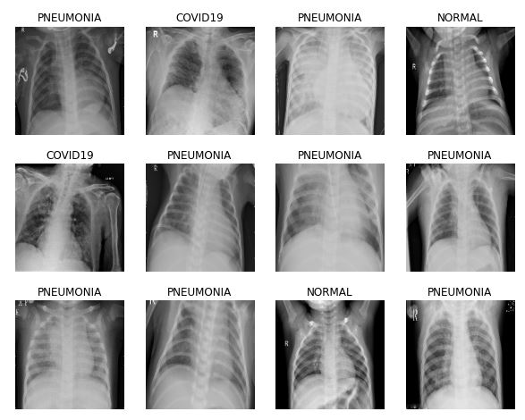
Dataset is organized into 2 folders (train, test) and both train and test contain 3 subfolders (COVID19, PNEUMONIA, NORMAL) one for each class. DataSet contains total 6432 x-ray images and test data have 20% of total images. As a start, it is very important to inspect the data across the three classes:

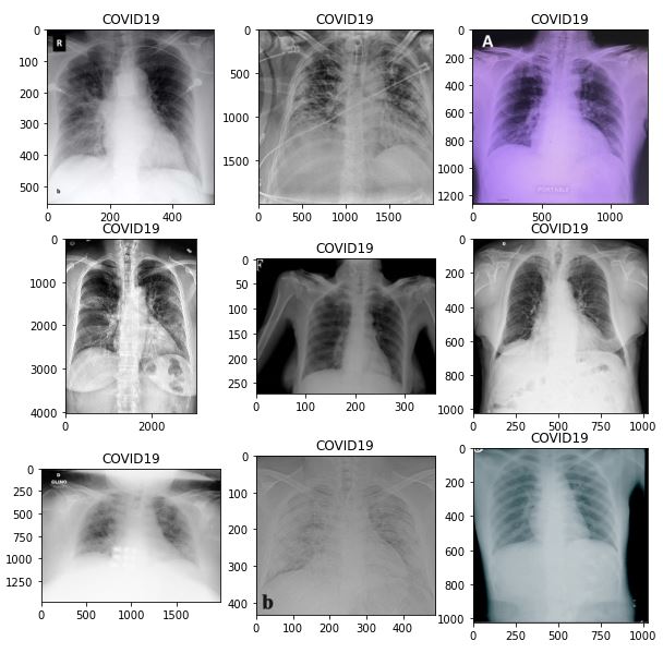
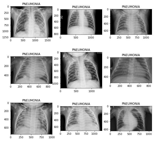
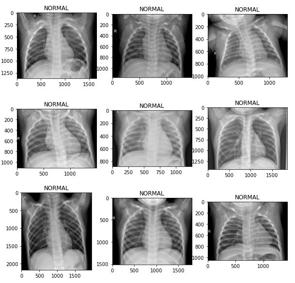
cov_sample PNEUMONIA_sample normal_sample

It is clear that images are at different sizes.

2) Data scaling, normalization and augmentation

Based on data inspection, images are scaled to a size of 244 by 244, normalized to values (0,1) and augmented by simple zoom and rotation to enhance the generalization.

image_size = 224 
BATCH_SIZE = 16 

data_path = '/kaggle/input/chest-xray-covid19-pneumonia/Data'

train_datagen = ImageDataGenerator(rescale = 1./255,
                                   zoom_range = 0.2,
                                   rotation_range=15,
                                   horizontal_flip = True)

test_datagen = ImageDataGenerator(rescale = 1./255)

training_set = train_datagen.flow_from_directory(data_path + '/train',
                                                 target_size = (image_size, image_size),
                                                 batch_size = BATCH_SIZE,
                                                 class_mode = 'categorical',
                                                 shuffle=True)

testing_set = test_datagen.flow_from_directory(data_path + '/test',
                                            target_size = (image_size, image_size),
                                            batch_size = BATCH_SIZE,
                                            class_mode = 'categorical',
                                            shuffle = True)

Accordingly, the dataset shape is as follows:

print("train batch ", training_set.__getitem__(0)[0].shape)
print("test batch ", testing_set.__getitem__(0)[0].shape)
print("sample train label \n", training_set.__getitem__(0)[1][:5])

train batch (16, 224, 224, 3)
test batch (16, 224, 224, 3)
sample train label [[0. 0. 1.] [0. 1. 0.] [0. 1. 0.] [1. 0. 0.] [0. 0. 1.]]

It is also important to understand the one-hot-encoding

training_set.class_indices

{‘COVID19’: 0, ‘NORMAL’: 1, ‘PNEUMONIA’: 2}

Testset sample after data preparation:

testset_sample

3) Training Tips

Callbacks

It is usually important to use callbacks while training. For example:

ReduceLROnPlateau: Reduce learning rate when a metric has stopped improving
EarlyStopping: Stop training when a monitored metric has stopped improving

lr_reduce = tf.keras.callbacks.ReduceLROnPlateau(monitor='val_loss', factor=0.5, epsilon=0.0001, patience=3, verbose=1)
es_callback = tf.keras.callbacks.EarlyStopping(monitor='val_loss', patience=5, verbose=1)

Label smoothing

Label smoothing is a mechanism for encouraging the model to be less confident. Instead of minimizing cross-entropy with hard targets (one-hot encoding), we minimize it using soft targets, this usually leads to a better generalization.

def categorical_smooth_loss(y_true, y_pred, label_smoothing=0.1):
    loss = tf.keras.losses.categorical_crossentropy(y_true, y_pred, label_smoothing=label_smoothing)
    return loss

Imbalanced data

In the case where data is (number of samples of some class is much more another class), different methods can be applied. Class weight is a simple method that can be used to specify sample weights when fitting the classifiers. For example, in the training data it is found that:

NORMAL: 1266
PNEUMONIA: 3418
COVID19: 460

Accoringly, class weights can be applied:

counter = Counter(training_set.classes)                          
max_val = float(max(counter.values()))       
class_weights = {class_id : max_val/num_images for class_id, num_images in counter.items()}

model.fit_generator(..., class_weight=class_weights)

Note: class weight is not used in the following experiments.

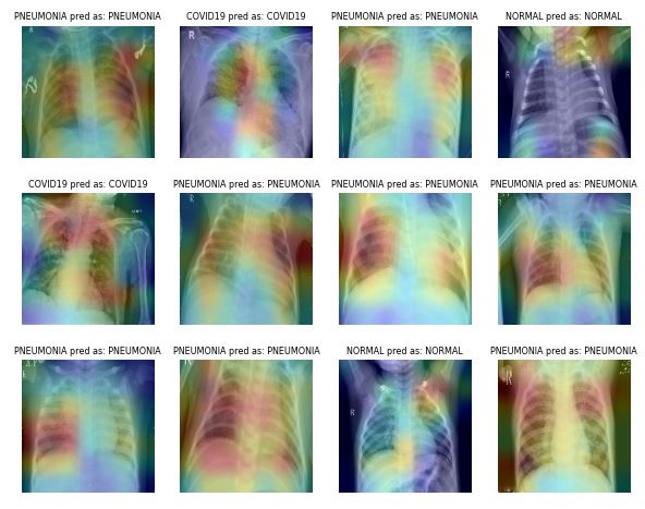
4) Understanding Results through visualization

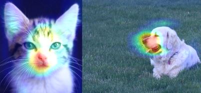
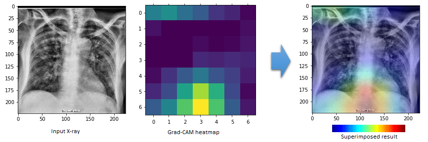
Class Activation Map (CAM) visualization techniques produce heatmaps of 2D class activation over input images, showing how important each location is for the considered class. In the paper Grad-CAM: Why did you say that? Visual Explanations from Deep Networks via Gradient-based Localization, the visualization is conducted by taking the output feature map of a convolution layer (given an input image), and then weighing every channel (feature map) by the gradient of the output class wrt the feature map.

cradcam

For example, the last CNN layer of some trained network has shape of 7 x 7 x n. Accordingly, we can find the corresponding 7 x 7 heatmap and generate the final result as shown below for the COVID19 test sample located at /test/COVID19/COVID19(164).jpg

cradcam2

5) Transfer Learning

Instead of starting from scratch, Transfer Learning is used by loading a generic and well trained image classification network for feature extraction, and then adding few layers (head) to be trained for the target task. Three pretrained networks are used:

Steps:

The pretrained network is loaded without the final classifcation head.
Freeze the weights of the pretrained network.
Add new head layers to be trained.

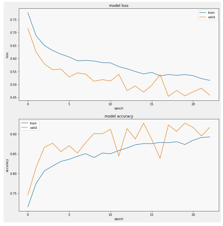
DenseNet201 Transfer Learning

pretrained_densenet = tf.keras.applications.DenseNet201(input_shape=(image_size, image_size, 3), weights='imagenet', include_top=False)

for layer in pretrained_densenet.layers:
  layer.trainable = False

x1 = pretrained_densenet.output
x1 = tf.keras.layers.AveragePooling2D(name="averagepooling2d_head")(x1)
x1 = tf.keras.layers.Flatten(name="flatten_head")(x1)
x1 = tf.keras.layers.Dense(64, activation="relu", name="dense_head")(x1)
x1 = tf.keras.layers.Dropout(0.5, name="dropout_head")(x1)
model_out = tf.keras.layers.Dense(3, activation='softmax', name="predictions_head")(x1)

model_densenet = Model(inputs=pretrained_densenet.input, outputs=model_out)
model_densenet.compile(optimizer=tf.keras.optimizers.Adam(learning_rate=0.0001),loss=categorical_smooth_loss,metrics=['accuracy'])
model_densenet.summary()

Trainable params: 1,106,179

history_densenet = model_densenet.fit_generator(training_set, validation_data=testing_set, callbacks=[lr_reduce, es_callback], epochs=30) 

testset_sample

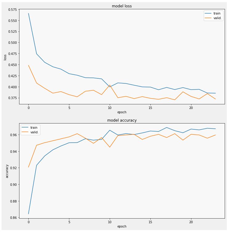
val_accuracy: 0.9596 (very good as a start indeed)

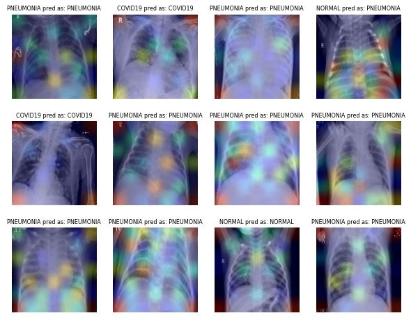
Sampe test results:

testset_sample

EfficientNetB7 Transfer Learning

pretrained_efnet = efn.EfficientNetB7(input_shape=(image_size, image_size, 3), weights='noisy-student', include_top=False)

for layer in pretrained_efnet.layers:
  layer.trainable = False

x2 = pretrained_efnet.output
x2 = tf.keras.layers.AveragePooling2D(name="averagepooling2d_head")(x2)
x2 = tf.keras.layers.Flatten(name="flatten_head")(x2)
x2 = tf.keras.layers.Dense(64, activation="relu", name="dense_head")(x2)
x2 = tf.keras.layers.Dropout(0.5, name="dropout_head")(x2)
model_out = tf.keras.layers.Dense(3, activation='softmax', name="predictions_head")(x2)

model_efnet = Model(inputs=pretrained_efnet.input, outputs=model_out)
model_efnet.compile(optimizer=tf.keras.optimizers.Adam(learning_rate=0.0001),loss=categorical_smooth_loss,metrics=['accuracy'])
model_efnet.summary()

Trainable params: 1,474,819

testset_sample

val_accuracy: 0.9169

Sampe test results:

testset_sample

Note that the defualt image size for the EfficientNetB7 is 600 by 600

VGG16 Transfer Learning

pretrained_vgg = tf.keras.applications.VGG16(input_shape=(image_size, image_size, 3), weights='imagenet', include_top=False)

for layer in pretrained_vgg.layers:
  layer.trainable = False

x3 = pretrained_vgg.output
x3 = tf.keras.layers.AveragePooling2D(name="averagepooling2d_head")(x3)
x3 = tf.keras.layers.Flatten(name="flatten_head")(x3)
x3 = tf.keras.layers.Dense(128, activation="relu", name="dense_head")(x3)
x3 = tf.keras.layers.Dropout(0.5, name="dropout_head")(x3)
x3 = tf.keras.layers.Dense(64, activation="relu", name="dense_head_2")(x3)
x3 = tf.keras.layers.Dropout(0.5, name="dropout_head_2")(x3)
model_out = tf.keras.layers.Dense(3, activation='softmax', name="predictions_head")(x3)

model_vgg = Model(inputs=pretrained_vgg.input, outputs=model_out)
model_vgg.compile(optimizer=tf.keras.optimizers.Adam(learning_rate=0.0001),loss=categorical_smooth_loss,metrics=['accuracy'])
# model_vgg.compile(optimizer=tf.keras.optimizers.Adam(learning_rate=0.0001),loss="categorical_crossentropy",metrics=['accuracy'])
model_vgg.summary()

Trainable params: 598,403

testset_sample

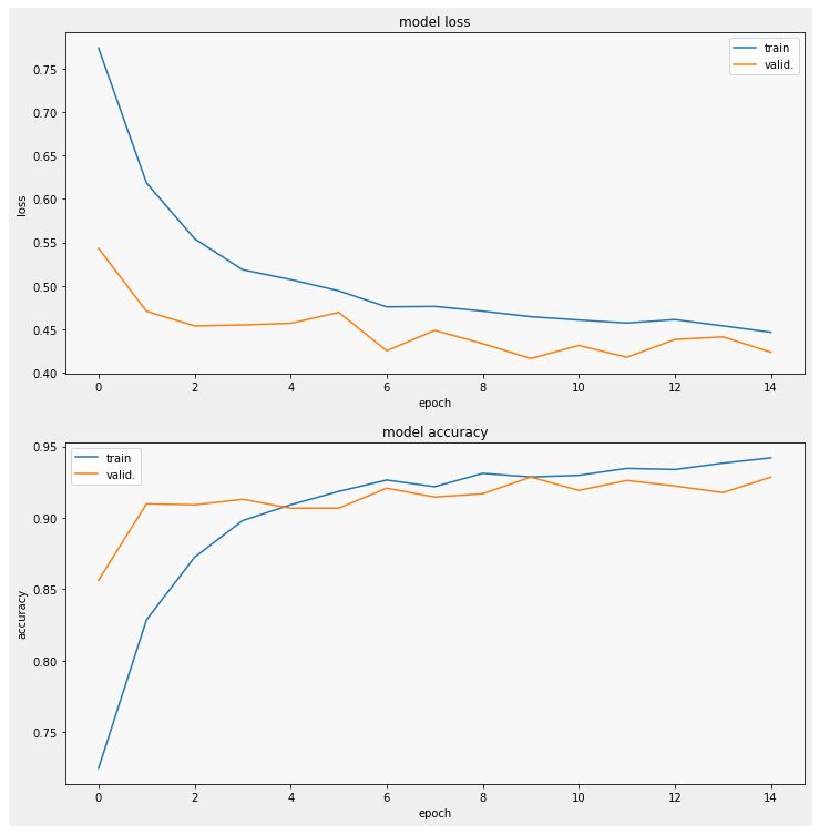
val_accuracy: 0.9286

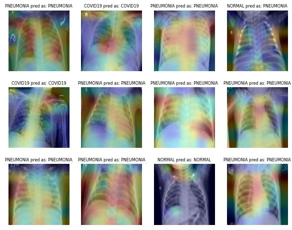
Sampe test results:

testset_sample

6) Ensemble Learning

In Ensemble learning, multiple models, such as classifiers, are combined together to improve the performance.

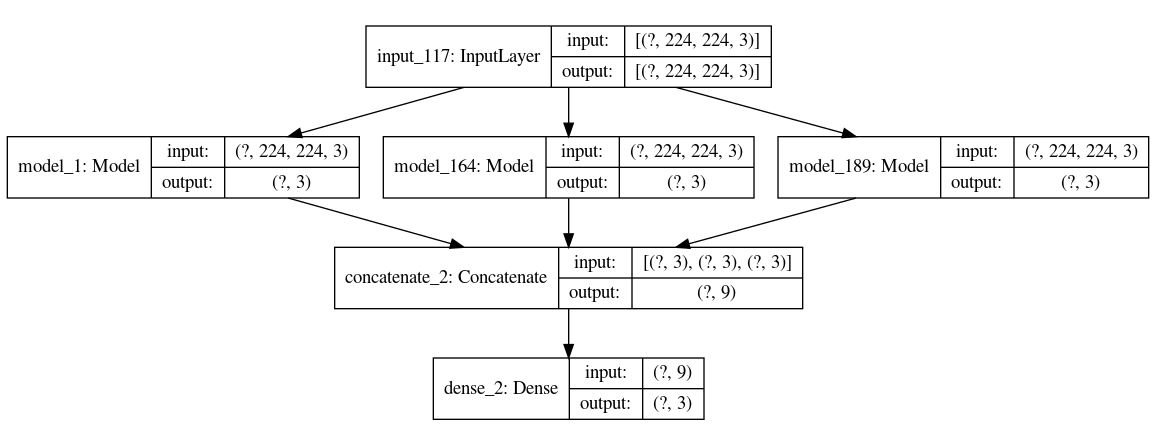
Ensemble at the probability level

In this setup, the network tries to find a combination of the final probs to come up with a better model. This is not the best way, but very simple where we have only 30 trainable parameters.

for layer in model_densenet.layers:
  layer.trainable = False

for layer in model_efnet.layers:
  layer.trainable = False

for layer in model_vgg.layers:
  layer.trainable = False

visible = tf.keras.layers.Input(shape=(image_size, image_size, 3), name="input")
x1 = model_densenet(visible)
x2 = model_efnet(visible)
x3 = model_vgg(visible)
merge = tf.keras.layers.concatenate([x1, x2, x3], name="concatallprobs")
model_out = tf.keras.layers.Dense(3, activation='softmax', name="predictions")(merge)

model_densenet_efnet_vgg = Model(inputs=visible, outputs=model_out)
model_densenet_efnet_vgg.compile(optimizer=tf.keras.optimizers.Adam(learning_rate=0.0001),loss='categorical_crossentropy',metrics=['accuracy'])
model_densenet_efnet_vgg.summary()

ens1

Ensemble at the last dense layer

This setup gives the network a better chance to learn from the dense layers before the softmax using only 579 trainable parameters.

model_densenet_nohead = Model(inputs=model_densenet.input, outputs=model_densenet.get_layer("dense_head").output)
model_efnet_nohead = Model(inputs=model_efnet.input, outputs=model_efnet.get_layer("dense_head").output)
model_vgg_nohead = Model(inputs=model_vgg.input, outputs=model_vgg.get_layer("dense_head_2").output)

for layer in model_densenet_nohead.layers:
  layer.trainable = False

for layer in model_efnet_nohead.layers:
  layer.trainable = False

for layer in model_vgg_nohead.layers:
  layer.trainable = False

visible = tf.keras.layers.Input(shape=(image_size, image_size, 3), name="input")
x1 = model_densenet_nohead(visible)
x2 = model_efnet_nohead(visible)
x3 = model_vgg_nohead(visible)
merge = tf.keras.layers.concatenate([x1, x2, x3], name="concatallprobs")
model_out = tf.keras.layers.Dense(3, activation='softmax', name="predictions")(merge)

model_densenet_efnet_vgg_nohead = Model(inputs=visible, outputs=model_out)
model_densenet_efnet_vgg_nohead.compile(optimizer=tf.keras.optimizers.Adam(learning_rate=0.001),loss='categorical_crossentropy',metrics=['accuracy']) #categorical_smooth_loss
model_densenet_efnet_vgg_nohead.summary()

ens2

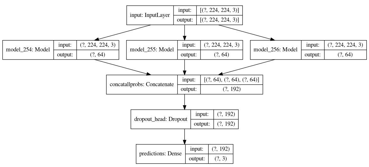
In this setup the final results are marginally better than any of the three models (there is still a room for enhancement)

Code

The full code can be found on Kaggle

7) Next Steps:

Use more versions of DenseNet EfficientNet
Use other nets such as MobileNet
Apply fine-tuning on some layers
Apply more reasonable data augmentation
Try Focal Loss with different settings
Consider that the cost of misclassification of normal as covid19 is not the same as misclassification of covid19 as normal

kaggle-COVID19-Classification

Chest X-ray (Covid-19 & Pneumonia)

Contents:

1) Data description

2) Data scaling, normalization and augmentation

3) Training Tips

Callbacks

Label smoothing

Imbalanced data

4) Understanding Results through visualization

5) Transfer Learning

DenseNet201 Transfer Learning

EfficientNetB7 Transfer Learning

VGG16 Transfer Learning

6) Ensemble Learning

Ensemble at the probability level

Ensemble at the last dense layer

Code

7) Next Steps: